
From Tokens to Bytes I: Scaling Hierarchical Networks
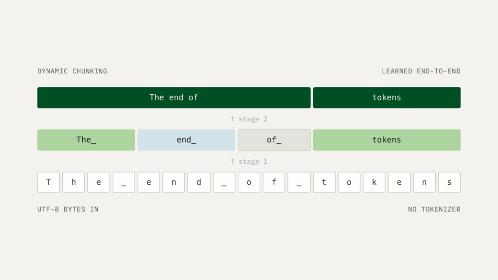
Since Richard Sutton’s influential essay in 2019, the concept of the bitter lesson has guided much of modern progress in AI. This concept espouses general methods that leverage computation and learn with scale, as free of human-engineered priors as possible. Our interpretation is that, fundamentally, intelligence is about learning from raw data: autonomously finding patterns, building abstractions, and developing meaning from messy low-level inputs, ideally end-to-end and as data-efficiently as possible. As AI advances into complex domains such as science, robotics, and biology – where data is scarce and often difficult for humans to understand, let alone engineer for – internalizing this philosophy to develop more general learning algorithms is more important than ever.
Language models are perhaps AI’s biggest success story today, and largely embrace the bitter lesson. Their abilities are largely attributable to scaling a few simple algorithms such as the Transformer architecture, next-token prediction, reinforcement learning, and test-time computation. However, they still rely on hand-crafted encoding steps such as tokenizers, which severely hinder their ability to learn end-to-end from the underlying data. Towards unlocking another step change of scaling, we believe that developing byte-level language models is foundational for AI progress – not just for improving standalone LLMs, but also as a litmus test for general learning methods. If we can’t even learn language well from characters and bytes, what right do we have to make progress on the next frontier?
In 2025, we developed the concept of hierarchical networks (H-Nets), which not only addressed tokenization in language models, but took a step toward even more general-purpose architectures that could learn from raw data across different modalities. We’ve since significantly improved the technology of H-Nets and are excited to share their capabilities! In this series of two posts, we’ll dig into new results and discuss the implications.
In this first post of a two-part series, we’ll explore scaling laws for H-Nets and their qualitative behaviors.
- We produce a standard scaling ladder for tokenized Transformers, and show that carefully controlled 1-stage H-Nets provide meaningful compute efficiency gains (up to 3-5x) purely through learned tokenization.
- We show empirical results from scaling up a more flexible 2-stage H-Net, where it outperforms a matched open-source model with extreme efficiency improvements (10x less compute and data).
- We analyze the patterns that H-Nets learn, where they show a rich diversity of new behaviors previously unseen in language models, such as in-context tokenization.
- We discuss how H-Nets go beyond language modeling, with ongoing research results in biology and vision, showing promise as a general architecture across modalities.
In the next post, we’ll do a deeper exploration of a larger range of models to understand better why H-Nets can be so much more efficient for language modeling.
Altogether, our results provide evidence that H-Nets are a foundational architecture that truly aligns with the bitter lesson, learning meaning directly from raw data and significantly improving efficiency and scalability. This research agenda represents a major opportunity to advance how AI can learn from all data, and we couldn’t be more excited to push the frontier!
Hierarchical Networks (H-Nets)
We introduced hierarchical networks (paper, blog) last year as a new end-to-end architecture that models multiple levels of abstraction in data, showing promise in language modeling and beyond. In a nutshell:
The terminology was inspired by the existing concept of chunking in cognitive psychology, which is an essential part of human intelligence. We believe it is also necessary for the frontier of artificial intelligence.
In the context of language modeling, the idea is to build new learning primitives that allow models to recursively chunk low-level data into higher-level meaning: characters into words, words into phrases, phrases into concepts.
In the context of this post, for the most part, one can think of hierarchical networks as replacing tokenization. Instead of pre-processing data from bytes into tokens (fixed chunks of bytes), H-Nets perform the chunking dynamically directly inside the model. Furthermore, the signature characterization of H-Nets is that they hierarchically perform this chunking end-to-end. In contrast, standard tokenized language models and even other alternatives (some of which we’ll see in Post II) employ multiple stages of training, and the process of chunking / tokenizing the data is performed entirely offline.
Details: Tokenization and BPE
Language models don’t read text directly but instead take as input a sequence of tokens from a fixed vocabulary. A natural vocabulary is the 256 byte values, producing one token per UTF-8 byte. Byte-level sequences, however, are long and expensive for standard language models to process. Tokenization aims to alleviate this problem by compressing the byte sequence into frequently occurring chunks. The most common approach, Byte Pair Encoding (BPE), starts from the 256 bytes and repeatedly merges the most frequent pair of adjacent tokens on a fixed training corpus, until the vocabulary reaches a set size (e.g. 128k for Llama-3). On our data mix, each BPE token covers about 4.57 bytes, making sequences much shorter than at the byte level. However, this compression is fixed, and tokenization remains one of the last parts of the language-modeling pipeline that is designed by hand rather than learned.
We’ll see in this post series that even in the narrower context of replacing tokenization, the end-to-end property of H-Nets provides real performance gains. Beyond tokenization, H-Nets have broad utility as a foundational architecture:
- H-Nets can be nested recursively, allowing for multiple levels of abstraction to be built. The main result of this post is a larger two-stage hierarchical network matched against an open-source baseline.
- H-Nets can operate over any type of data, not just bytes, and not just discrete data. In contrast, tokenizing continuous data is a serious challenge. In the final part of this post, we’ll preview some future research applying H-Nets beyond text.
H-Net architecture
Two-stage byte H-Net
Decoder
Decoder
Main network
Encoder
Encoder
Figure 1 illustrates a 2-stage H-Net and defines the main components of the model: the encoder, main network, and decoder. We sometimes call the encoder/decoder together the outer networks and the main model the inner network.
Throughout this post, we show results with a much improved version of H-Nets, which we plan to release. We’ll comment more on differences from the earlier architecture later in this post.
Part 1: BPE and H-Net Scaling Ladders
As with many architecture papers, the original paper on hierarchical networks focused on tuning language models of particular fixed sizes and data horizons (e.g. ~1.3B-parameter models on 100B tokens from FineWeb-Edu have been very common). Although they looked very promising, a missing piece was the lack of compute-optimal scaling laws, now a standard way to measure pretraining innovations. For example, Kimi’s popular innovations on Kimi Delta Attention (KDA) and attention residuals measured compute multipliers of 1.16x and 1.25x, respectively.
In order to validate the gains of our improved H-Net architecture, we first set out to build a modern LLM scaling ladder, and then replaced its tokenization components with a carefully controlled hierarchical network.
- We set up a training mixture for comparing byte-level and BPE scaling laws on equal terms, carefully matching the processing and even re-training a BPE tokenizer for the baseline.
- We set up a scaling ladder for a baseline BPE Transformer language model according to standard practices, reproducing results from the literature.
- We then converted each rung to a byte-level H-Net as a drop-in replacement, reusing the BPE backbone architecture and hyperparameters.
This recipe directly showed stronger results on validation loss (1.3x), with gains increasing on subdomains such as code (2x), as well as improving out of distribution (2x on evaluation, and up to 5x on out-of-domain code).
A data-controlled comparison
Since byte-level and BPE models process the same data at different granularities, extra care is needed to keep the methodology controlled.
Data mixture: Our training dataset consisted of 70% English, 20% code, 5% math, and 5% multilingual, measured by the number of bytes.
Data processing: Every sample is processed as both bytes and BPE tokens, splitting at the same boundaries; both byte- and BPE- processed datasets therefore contain exactly the same text with aligned document boundaries.
Metric: We use the standard bits-per-byte (bpb) metric for measuring next-token prediction loss in a way normalized between different tokenizers.
In-corpus BPE tokenizer: LLMs generally use off-the-shelf BPE tokenizers; an advantage of H-Nets is that they learn their chunking directly on the training distribution. To be extra careful, we also trained a BPE tokenizer on the corpus. We used this for the BPE scaling laws below, which ended up resulting in about a 1.1x compute gain on both validation loss and downstream evals (so the H-Net would have an even greater compute multiplier against a standard off-the-shelf tokenizer!).
The BPE tokenizer’s vocab size is 128k, matching the Llama-3 tokenizer that we were working off of. The in-corpus tokenizer compressed the dataset slightly more, increasing the average BPE token length from 4.45 (Llama-3 tokenizer) to 4.57. Measured in tokens of the in-corpus BPE tokenizer, the training dataset comprised 64.7% English, 23.7% code, 6.1% math, and 5.5% multilingual.
Bytes per BPE token
Target mixture 4.57
Creating a robust BPE baseline
For our baseline, we fit a well-tuned scaling law for a standard BPE Transformer. To do this, we constructed a scaling ladder, following modern scaling recipes such as Kimi and MAI, fully defining a family of models by the number of layers L. We set the hidden dimension D to a multiple of 128 such that the aspect ratio D/L is approximately 75. For all models, we use multi-head attention with the number of heads equal to the number of layers and a fixed head dimension of 128. For the MLPs, we use SwiGLU layers with the intermediate dimension set to 3.6D, again rounding to the nearest multiple of 128.1
| Model | Total params | Backbone params | Layers | Hidden dim | Attn heads | Head dim | FFN dim |
|---|---|---|---|---|---|---|---|
| L08 | 221M | 56.4M | 8 | 640 | 8 | 128 | 2304 |
| L12 | 399M | 169M | 12 | 896 | 12 | 128 | 3200 |
| L16 | 673M | 378M | 16 | 1152 | 16 | 128 | 4096 |
| L20 | 1.22B | 822M | 20 | 1536 | 20 | 128 | 5504 |
| L24 | 1.81B | 1.35B | 24 | 1792 | 24 | 128 | 6400 |
| L28 | 2.62B | 2.10B | 28 | 2048 | 28 | 128 | 7424 |
We then fit compute-optimal scaling laws with the standard iso-FLOP sweep methodology.
- All runs use the Muon optimizer and WSD learning rate schedule with fixed-fraction warmup and decay.
- We tuned batch size and learning rate on selected rungs and fitted hyperparameter scaling laws to extrapolate to larger ones.
- We counted FLOPs carefully in all models, including all sequence-mixing layers and the LM head. For softmax attention, we also count only causal FLOPs, as, due to the quadratic complexity, over-counting non-causal FLOPs penalizes byte-level models which process longer sequences.
An equivalent H-Net ladder
Because H-Nets over bytes are so different from standard tokenized models, it’s highly nontrivial to compare them directly. There are so many moving parts: how many stages of chunking, the respective compression rates, the architecture configurations of each stage (outer vs. inner networks), and the hyperparameters for each component.
We decided to investigate a narrower setting: how do H-Nets compare against BPE models, if restricted to being interpreted as purely replacing the tokenization portion of the language model?
To do this, we converted each rung of the BPE ladder to a byte-level 1-stage H-Net. A 1-stage H-Net can be viewed as a standard language model with learned tokenization: the inner network operates over chunks (which play the role of tokens) and the outer networks perform the role of dynamic tokenization, encoding bytes into chunks and decoding them back. Each rung is matched very carefully:
- The H-Net’s inner network is exactly the same Transformer architecture.
- The H-Net’s outer network (encoder and decoder) is FLOP- and parameter- matched to the tokenization layers (embedding and “unembedding” or projection head).
- The H-Net’s compression ratio is matched to the BPE compression rate (4.57) by using a strong auxiliary loss.
- The BPE Transformer’s hyperparameters (batch size and learning rate) are directly transferred.
Converting a BPE rung into an H-Net
One rung of the ladder
Compute multipliers: validation, downstreams
Compute-optimal scaling laws
Byte H-Net vs. BPE Transformer
1018101910201021Compute (FLOPs)Loss (BPB)0.650.700.750.800.850.900.951.28×
1018101910201021Compute (FLOPs)Loss (BPB)1.11.21.31.41.83×
1018101910201021Compute (FLOPs)Loss (BPB)0.80.91.01.11.21.32.06×
Byte H-NetBPE Transformer
At all model sizes, the H-Net run achieved lower loss than the matching BPE Transformer rung – the “dynamic tokenization” interpretation outperformed the static tokenizer out of the box!
After fitting compute-to-loss power laws to both ladders, we can compare the compute efficiency of both architectures, quantified by how much less compute the H-Net takes to reach the same loss as the BPE ladder (Figure 4).
In-domain: The H-Net is 1.28x more compute efficient than the BPE Transformer.
Evaluations: We examined standard downstream evaluation suites such as Paloma and OLMES, each of which consists of a mixture of dozens of datasets and tasks spanning human languages and domains (code, math, etc.). For each one, we measured the “soft accuracy” of a model as the bits-per-byte it assigns to the correct answer. Re-fitting compute-to-bpb scaling laws to each suite, we see that the gap between H-Nets and BPE Transformers grows further to around 2x.
In the second post of this series, we analyze the out-of-distribution behavior of a range of language models more deeply, providing support for the hypothesis that more flexible and semantic chunking leads to stronger downstream transfer.
Compute multipliers: code
Interestingly, H-Nets particularly excel on code. Fitting the same laws to each programming language it was trained on, the H-Net’s compute multiplier rises for all 15 languages: from 1.49x on Markdown to 2.40x on Go, with a median of 2.04x (Figure 5).
The gains are larger still on languages outside the training mix. On ten Stack v2 languages that were not part of the data mix, including OCaml, Prolog, Lean, and Fortran, H-Net’s multiplier rises to a median of 3.10x, from 2.19x on Haskell to 5.37x on Prolog.
(Why is this important? LLMs are often asked to work with code they may not have seen much data for, and are increasingly used to invent or reason over new languages such as DSLs, kernel programming languages, and hardware abstraction layers. So OOD code performance may actually be quite meaningful to frontier models.)
Compute efficiency gain on code
1 / 15
Byte H-NetBPE Transformer
Intuitively, we hypothesize these phenomena arise for a few reasons:
- H-Nets perform better on new distributions in general because they learn how to create semantic concepts from lower-level data, which generalize better. This is reflected in the rise from in-distribution (1.28x) to downstream evaluations (2.06x), and from in-domain programming languages (median 2.04x) to out-of-domain programming languages (median 3.10x). Post II will discuss out-of-distribution transfer in much more detail.
- H-Nets are better on data that’s difficult to tokenize, in the sense of lacking a small vocabulary of reusable patterns. This is particularly evident in code, which is very dynamic and possesses a wide range of whitespace and symbols, syntax structure, and variable names (essentially an infinite vocabulary even over Latin characters!). Pre-defined tokens are less likely to capture the full range of semantics.
- In Part 3, we show that H-Nets learn semantics on the fly at inference time, for example being able to learn variable names in code as one token; we hypothesize this is one particular mechanism that lets them excel at code.
Finally, we make the interesting observation that the H-Net’s improved performance on code is not due to spending additional compute.
Compression by data source
H-Net compresses moreH-Net compresses less
Figure 6 supports our thesis that language modeling ability is not just about compute and parameters, but learning the right meaning from the data. By finding semantic chunks from raw bytes, H-Nets perform much better on difficult-to-tokenize domains while spending less compute.
Limitations of the H-Net ladder
Controlling H-Nets to match BPE-tokenized models in the way we did is actually seriously restrictive. Hierarchical networks have a tremendous degree of flexibility:
- They can involve multiple stages of chunking, compared to a single static phase by BPE.
- The compression rates are freely controllable; equating them to the ratio defined by BPE is actually against the spirit of H-Nets, which ideally should find natural compression rates of the data (loosely governed by information content and semantics of the data).
- The hyperparameters of each network should be tunable; in fact, we’ve found that setting them equal to a BPE model is suboptimal.
Importantly, the H-Net ladder we defined by changing just the tokenization part of a BPE Transformer is not an optimal H-Net architecture at all. In fact, it can be viewed as being very favorable to the BPE Transformer baseline. What happens when we remove these restrictions?
Part 2: Training a larger H-Net
Data efficiency vs. SmolLM3
02468101252545658606264Training tokens (T)Average score, six tasks (%)0.000T tokens
Byte H-NetSmolLM3-3B (BPE Transformer)
We aimed to scale H-Nets up larger than the scaling ladders and the earlier versions (the first paper trained up to the equivalent of a 1.3B parameter model for 100B tokens). As a baseline, we chose SmolLM3, a 3B Transformer LLM released by Hugging Face with a fully documented training recipe. Because the SmolLM3 team released the model architecture, the training datamix, and several checkpoints throughout the training run, we were able to reproduce the recipe and compare the models throughout the training process – including past the horizon we trained to!
Data: SmolLM3’s pretraining consisted of three phases with 8T/2T/1T tokens, using the Llama-3 tokenizer, for a total of 11.1T tokens. As our target horizon was much shorter, we used only the stage-1 data mixture. We made a best-effort reproduction built from the same public sources. Controlling for data is subtle; most training recipes report their data mixture as a fraction (e.g. SmolLM3’s is 73.2 / 12.1 / 12.0 / 2.7 for English web / multilingual / code / math), but this is usually in tokens. To try to control for data properly, we decided to match the underlying byte-level mixture (just as we did for the scaling ladders), which ended up being 76.5 / 10.9 / 10.3 / 2.2.
Optimization: We match the baseline identically without additional tuning for the H-Net: AdamW (0.9, 0.95), weight decay 0.1, clipping 1.0, peak LR 2e-4, same WSD schedule with 5B token-equivalents of warmup. We cooled down for the last 15% of training; one difference from the baseline is that SmolLM3’s cooldown phase appeared during its 3rd pretraining stage (after 10T tokens), with a different data mixture.
Architecture: We built a two-stage hierarchical network over bytes.
- The outermost (byte-level) stage uses four Mamba-2 layers in the encoder and four in the decoder.
- The next stage adds a sliding-window attention block and four more Mamba-2 layers on each side.
- The main network is a 40-layer Transformer with the same per-layer shape as SmolLM3, with global attention in every layer.
- The compression ratios were set according to prior work (targeting 4x and 2x in the two outer encoder stages).
Where are the FLOPs spent?
Unlike the scaling ladders, we focused more on aligning with the philosophy of hierarchical networks: allowing the model to perform dynamic chunking in multiple stages, ideally following the semantics of the data. This made matching all axes to the baseline impossible, as parameters and compute get spent in very different ways. We aimed to control for FLOPs/byte, so that every minibatch of training sees the same underlying data and spends the same amount of compute as the baseline.
- The compression ratios were set so the main network sees roughly one position for every 8 bytes (the trained model ends up at ~7.6×). Compared to ~4.5 bytes per Llama-3 token, this is about 40% fewer tokens than SmolLM3 processes on the same text.
- That saving trades off for the outer encoder/decoder stages, which account for about 43% of the H-Net’s FLOPs (compared to 8% for the embedding and LM head in the tokenized Transformer).
- The resulting models are compute matched to within 2% FLOPs/byte.
The H-Net’s total parameter count ended up at 3.67B, against 3.08B for the baseline. The difference is mostly the encoders and decoders plus the four extra main-stage layers; the byte embedding is tiny.
Parameters and FLOPs per component
H-Net vs. SmolLM3
Results
We evaluated using benchmarks and the same evaluation suite as the official SmolLM3 results, among their set of “Reasoning & Commonsense” and “Knowledge & Understanding” evaluations.
Figure 7 shows both models’ benchmark scores over training. The H-Net reaches SmolLM3’s final average score after ~1T tokens compared to ~11T tokens. Since the two models are compute-matched per byte, the saving in training FLOPs is proportional.
Discussion: Data controls
Despite our effort to control for data and compute fairly, in hindsight we realized it’s still not obvious what a proper methodology should be. For example, let’s look at English vs. code: the reason SmolLM3’s token mix of 73.2% / 12.0% respectively becomes 76.5% / 10.3% at the byte level is because tokenizers compress English more (see Figure 8b), which itself is an artifact of BPE tokenization (it spends more effort compressing more frequently appearing data, so it’s tied to the arbitrary data distribution).
On the other hand, the philosophy of H-Nets is to compress data according to an “intrinsic” notion of compressibility and semantics. For example, we find that H-Nets compress code a lot more because code is naturally compressible; and we attribute much of H-Net’s improvements on code to this ability to understand the data better. But at the same time, this means that H-Nets spend less compute on code (because the same piece of code data gets turned into far fewer chunks sent into the main network) relative to the BPE baseline! So would a better way to control it be to let the models spend similar amounts of compute per source instead?
In short, BPE models and H-Nets can compress subdomains in opposite ways – for example, BPE compresses code less than English while H-Nets compress it more – so it’s impossible to both data- and compute- match, and the right way to compare models is subtle. These are all open research problems!
Compression and compute per source
Sort by
H-Net compresses more or spends lessH-Net spends moreEqual to SmolLM3
Hover over a source to see its numbers.
Part 3: Qualitative analysis of learned behaviors
Training dynamics
We show how the H-Net learns from the beginning of training, continually updating its representations on a particular held-out piece of text (the abstract from the original H-Net paper!).
Chunking over training
Held-out text
step 71,856 · 671.0B bytes
H-NetH-Net abstract · 208 chunks · 8.4 bytes each
Chunks in this textStage 0Stage 1
Visualizing H-Net’s dynamic tokens
We show an H-Net’s chunks for several examples (that it was not trained on) for every source of its data mixture. We also show various baselines including three BPE tokenizers:
- the Llama-3 tokenizer (which SmolLM3 uses)
- a new BPE tokenizer trained directly on the SmolLM3 training corpus, to show what BPE would learn completely in-distribution (Corpus)
- an in-corpus BPE tokenizer with no pretokenization (Corpus (NP)), which we will cover more in the next post
We also provide chunks of the originally published H-Net (denoted LH-Net) to illustrate qualitative improvements from our internal version.
Language
H-Net
Compare with:
Figure 10a shows examples from human languages.
- H-Net presents coherent and semantically meaningful boundaries for natural languages including Latin-based/Germanic languages that use spaces as delimiters, as well as multi-byte character languages (e.g. CJK, Hindi) with and without explicit delimiters.
- H-Net merges multiple words into a single chunk that can be naturally grouped together. For example, “a foot”, “quite a few”.
- Interestingly, tokens from the BPE tokenizer without pretokenization also often comprise multiple words. However, they exhibit many weird boundaries, such as
beat a bearbeing separated intobeat abear.
- Interestingly, tokens from the BPE tokenizer without pretokenization also often comprise multiple words. However, they exhibit many weird boundaries, such as
- H-Net boundaries are not pattern-based. Rather, they are context-based. For example, while “a” frequently gets merged with the following noun in English,
aless frequently is grouped with other words in Italian as it has different meanings. - For all languages, H-Net achieves much higher compression than BPE tokenizers. This is more pronounced in certain languages that require many bytes to form a character such as Hindi.
Code
H-Net
Compare with:
Figure 10b shows examples from programming languages.
- H-Net boundaries for coding languages also exhibit interesting characteristics derived from their context-based properties. For instance, BPE tokenizers strictly use newline as a boundary, whereas H-Nets accept multi-{space/tab/newline} chunks (example:
__init__(n self,). - H-Nets can generally compress code far more than BPE (also see discussion for Figure 8b).
- H-Nets can benefit from in-context tokenization to recognize repeated motifs such as new variable/function names as they keep recurring.
Aside: How does this compare to the original H-Net?
Since we published the concept of hierarchical networks in 2025, we’ve made many significant improvements to the core architecture and learning mechanisms. We plan to release some of these architectures to the community over time. Here we discuss some concrete qualitative areas of improvement.
For the purposes of this comparison, we’ll call the earlier model the LH-Net, where L can be thought of as meaning “lazy” or “lookahead”. In brief, this original model aims to draw chunk boundaries only after it sees the start of the next chunk.2 This allows LH-Net to have more context in creating chunks, but turns out to negatively impact its ability to perform next-token (byte) prediction as well as model multiple hierarchies.
Qualitative differences between LH-Net and our current internal H-Net can especially be seen when examining recursive hierarchical networks with multiple stages.
- In English, consider the first example.
- Stage 0 chunks from H-Net are generally more meaningful than LH-Net’s. For example, when they occur in the middle of English words, they generally align better with linguistically meaningful stems.
- H-Net examples:
trackers→trackers,wondered→wondered,nearby→nearby - LH-Net examples:
rhino→rhino,from the fact→from thefact,mass→mass,Over→Over,ethical→ethical
- In scripts where characters are represented with multiple bytes, such as CJK (Chinese, Japanese, Korean), a multistage LH-Net doesn’t segment characters correctly, even after both stages of chunking.
New emergent behaviors: in-context tokenization
In-context tokenization
An H-Net’s tokenization not only changes over training time, but can also evolve during inference, which we call in-context tokenization. We previously discussed some simple cases of how boundaries of H-Nets are context-based, and not pattern-based. In Figure 11, we highlight four interesting examples of the in-context tokenization:
- New concepts: When an H-Net encounters an unfamiliar word or a new concept, it tends to split the word into multiple chunks (similar to how BPE would read unfamiliar strings). As it encounters the same word multiple times, it progressively learns to group the word into fewer chunks.
- Repeated formats: If there is a repeating phrase, we can easily expect what would come next. Similarly, in such a scenario, H-Nets learn to further compress inputs, drawing very large chunks to conserve compute.
- Recurring motifs: As shown in the figure, H-Nets learn to discover implicit patterns in inputs. In the letter blocks example, the recurring blocks –
LURD,WHYV, andFYB– get grouped together. The digit blocks example is an interesting case that shows how an H-Net can discover the repeated motifs (2526,3987, and3526) underlying the data. The behavior of stage 0 vs. stage 1 is also interesting to observe.
H-Net
Compare with:
Out-of-domain Programming Languages
Finally, we visualize how H-Nets handle programming languages that they haven’t seen. We saw previously that the H-Net ladder was particularly effective (relative to the baseline) for out-of-domain programming languages. Figure 12 shows examples from these 10 programming languages.
H-Net
Compare with:
Part 4: From tokens to atoms: hierarchical networks beyond language
This post has so far focused on the capabilities of hierarchical networks as applied to language modeling on bytes, which captures the ideal of learning from raw data in the context of language.
We believe that the utility of H-Nets goes far beyond language: the core concept of chunking low-level data into higher-level patterns is fundamental to intelligence, and can be applied to any domain.
One such area is audio, a core focus of Cartesia, where the inability of models to autonomously abstract raw audio into phonemes and words represents a major bottleneck toward multimodal speech-to-speech models (and in fact was a motivation for us to start investigating H-Nets years ago!).
More broadly, bytes are not necessarily a universal encoding for all domains. Most domains have a concept of “primitive building blocks”, such as characters or bytes for language, pixels for images and video, waveforms for audio, nucleotides for biology, and so on. We’ve started thinking of different modalities as being built from various base atoms, and of so-called atomic models as the truly bitter-lesson-pilled way to build powerful foundation models for multimodality. We highlight some examples of additional domains.
Biology (DNA)
DNA is the lowest-level programming language of biology. Depending on the context, its natural level of abstraction, and therefore its natural primitive units, changes drastically. Because of this, we hypothesized that H-Net’s dynamic tokenization would be significantly more effective than a static tokenization scheme on the DNA domain.
DNA scaling ladder
We compare an H-Net and a Transformer on autoregressive modeling of DNA sequences. Both models operate at the nucleotide resolution as input (so the vocabulary size is 4, plus some special token IDs). The H-Net has a target compression ratio of 6×: its main network sees approximately one chunk for each six nucleotides.
We fit compute-optimal scaling ladders using a similar procedure as in Part 1. The H-Net leads to a 6–7× compute gain on all three sets.
Details: DNA Datasets
- Training data. The GTDB set of prokaryote genomes from OpenGenome (stage 1), approximately 274 billion nucleotides. We cut each contig into segments of 8,192 nucleotides or less, and we mix the segments.
- Validation set. 8,192 segments that we keep out of training (approximately 56 million nucleotides). Other segments of the same genomes are in the training data.
gtdb_valid_smallandgtdb_test. The two official held-out sets of OpenGenome: 5 contigs (26 thousand nucleotides) and 50 contigs (374 thousand nucleotides). All of these contigs come from one genome. We do not train on these contigs, but other contigs of this genome are in the training data.
Compute-optimal scaling on DNA
H-Net vs. Transformer
1018.510191019.510201020.5Compute (FLOPs)Loss (BPB)1.31.41.51.61.75.95×
1018.510191019.510201020.5Compute (FLOPs)Loss (BPB)1.501.551.601.651.701.755.83×
1018.510191019.510201020.5Compute (FLOPs)Loss (BPB)1.41.51.61.77.06×
H-NetTransformer
Qualitative analysis in DNA: Biology’s context-dependent atomics
H-Net was trained only on the next-letter prediction task for prokaryote (bacterial and archaeal) genomes, so the adherence of H-Net’s token segmentation to biology’s natural structure in the human genome is purely emergent behavior. Here we display some of these examples:
H-Net chunksHuman chromosome 6, histone gene H2BC17 · never seen in training
one chunk per band1st letter of a codon2nd letter of a codon3rd letter of a codonstart / stop codonpromoterhairpinend of the RNA
86 chunks in 680 letters · 7.9 letters each
Quick primer on Biology/DNA
DNA and genes. DNA is a string of four letters: A, C, G, and T. A gene is the stretch of DNA responsible for producing an RNA sequence, which is usually translated into a protein. Only its coding region actually spells out the protein, while the DNA around it is far less constrained and more information-sparse: the promoter region before it, the signal that ends the RNA after it. They control when and how the protein is made, not what it is. Additionally, in human genes, introns, non-coding regions that sit in the middle of the coding region, are spliced out and also do not contribute to the protein sequence.
Codons and the reading frame. The coding region is read three letters at a time, from a start codon (usually ATG) to a stop codon (TAA, TAG, or TGA). Each three-letter codon names one amino acid in a protein sequence. Where reading starts sets the reading frame: shift it by one letter and every codon downstream changes.
Some notable learned behaviors:
- Inside a gene, the H-Net router settles on a different atomic unit depending on what it is reading; we see biologically aligned treatments of:
coding region vs. non-coding
regionsexons vs. introns
Robustness: H-Net’s learned codon
grid isn’t fixed; where two coding regions overlap and the second is offset,
H-Net’s boundaries adapt quicklyIn a transfer RNA (tRNA) gene, the
natural unit shrinks to a single letter. H-Net boundaries learn to adhere to
this new natural unitLarge sections of repeats in DNA
are typically information-sparse, so in a repeat, the natural biological unit
grows to the whole repeat
expect, a lot of these biologically adherent behaviors aren’t learned until late
into training, as shown through the learning trajectory animation. The late
onset of these behaviors highlights the nontriviality of the “tokenization task”
in the DNA domain, and supports the thesis that hand-crafted tokenization
schemes would be even more difficult and less effective in multimodal domains
than in language.
Vision
Hierarchical networks are naturally defined for one-dimensional sequential data, where chunking and segmentation are intuitive. Extending them to higher-dimensional modalities, however, presents a significant technical challenge – and simultaneously a great opportunity, as vision is a domain naturally suited to hierarchies. In ongoing research, we’ve developed new techniques to apply H-Nets to N-dimensional data such as images and videos. When integrated into a pixel-space diffusion model, H-Nets not only improve generation quality, but also uncover unsupervised semantic concepts directly from raw data – mirroring the emergent behaviors we saw with language.
In more detail, we take a standard pixel-space flow-matching baseline JiT, and replace its backbone with a multi-dimensional H-Net. Just as with 1D H-Nets, the model learns both where to chunk and how much to compress. This allows it to dynamically reallocate compute across three axes: spatially (focusing on detailed regions over simple ones), integration time (varying effort by denoising step), and samples (allocating more compute on complex images). Consequently, the model consolidates homogeneous or low-information areas and focuses on salient details, and discovers semantic segmentations of the image completely without supervision. A final interesting detail is that unlike existing token-merging methods that rely on the similarity of contiguous patches, our 2D H-Net doesn’t enforce local grouping. Because of this, the model often appears to infer underlying 3D structure from flat 2D projections. For instance, it routinely groups disjointed background regions into a single coherent chunk, even when they are separated in the image by occluding foreground objects.
Learned chunks on images
Held-out images
Next: Post II
In the next post, we dig into the compute efficiency results in much more detail. We study loss-to-loss scaling laws and find empirical evidence that H-Net’s improved performance really does come from its ability to learn from raw bytes end-to-end.
Citation
Please cite this work as:
Cartesia Research, "From Tokens to Bytes: Scaling Hierarchical Networks", Cartesia Blog, October 2026.Or use the BibTeX citation:
@article{cartesia2026hnet,
  author  = {{Cartesia Research}},
  title   = {From Tokens to Bytes: Scaling Hierarchical Networks},
  journal = {Cartesia Blog},
  year    = {2026},
  month   = {October},
  note    = {https://www.cartesia.ai/blog/from-tokens-to-bytes-part-1}
}