Educating a World Model to Play Pokémon

I feel a number of the most fascinating work occurring within the subject of Artificial Intelligence surrounds global community fashions. There are many sorts of global community fashions (and the time period itself has develop into a bit overloaded), however one of the crucial thrilling architectures for global community fashions is Yann LeCun’s JEPA (Joint Embedding Predictive Architecture). There are many variants, and one which caught my eye particularly was LeWorldModel. It appeared sufficiently small to coach regionally on my RTX 3080 Ti and had a less complicated design than most of the earlier JEPA architectures.
San Francisco has been lined in Pokémon memorabilia–large ads that includes most of the 1026 pocket monsters plastered throughout the subway strains and bus stops on Market Street. SF was the positioning of the Pokémon World Championships this 12 months, and plenty of eclectic and joyous Pokémon trainers might be discovered wandering the temperate hills and concrete monetary district of downtown SF. Maybe all of the ads had subliminally managed me, however I had determined {that a} good “global community” for our global community mannequin can be the 1996 recreation that began all of it, Pokémon Red.
The mechanics of Pokémon
Pokémon Red is a recreation the place you discover a global community, accumulate creatures known as Pokémon, and use them in battles.
You use the path buttons to stroll round or transfer by menus. The A button interacts with issues, advances dialogue, and confirms selections; the B button often cancels or backs out. Choosing a starter means approaching a Poké Ball (a container that holds Pokémon) and getting by the dialogue that confirms your alternative.
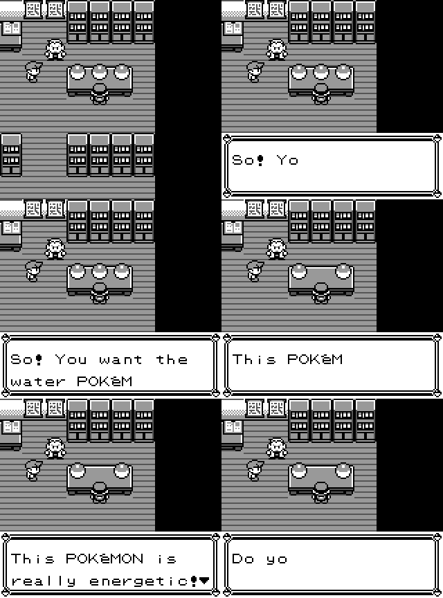
Near the start of the sport, the participant is inside Professor Oak’s lab, the place he gives you your first Pokémon: Bulbasaur, Charmander, or Squirtle. These are the three “starters,” every ready in a Poké Ball on a desk in his lab.
The GIF above is the ultimate results of the mannequin coaching: the mannequin deliberate a sequence of button presses that chosen Squirtle. There have been extra difficulties and setbacks than I anticipated, regardless that the mannequin had regarded promising in easier exams.
The Plan
The purpose was comparatively easy: defeat Professor Oak’s grandson. Breaking it down into a number of steps, I got here up with:
- Get to Professor Oak’s Lab
- Finish Dialogue with Oak
- Select a Starter Pokémon
- Try to exit the lab
- Face and beat Oak’s grandson
It rapidly got here to my consideration that this may be formidable for a primary experiment–so I narrowed it right down to choosing a starter from a saved state in Oak’s Lab, the place buying any of the three starters would depend as a profitable try.
From the saved place within the lab, having the mannequin press A twelve instances is sufficient. But can the mannequin be taught that? The mannequin may additionally simply wander round aimlessly, possibly in perpetual torment inside Oak’s lab. Or the mannequin may press B after each few sequences of A, cancelling its effort when it virtually reached its purpose.
What Even is a World Model?
A global community mannequin is a mannequin wherein we start with some present state or remark, and a few motion occurs that modifies this state, producing a brand new remark. Realistically, there must be some kind of correlation or hopefully causation between the motion on some state and the brand new state it produces. The purpose of the global community mannequin is to be taught this correlation. Let’s say the present remark is a screenshot of Professor Oak’s lab, with the participant in entrance of the Poké Balls, and the motion is urgent left, transferring the participant one tile to the left–producing the brand new finish screenshot. The purpose can be for the global community mannequin to develop some type of instinct that urgent left strikes the participant left.
$$
o_{t+1}approx F(o_t,a_t).
$$
Here (o_t) is the present screenshot, (a_t) is the button pressed, and (F) is the operate the global community mannequin learns to foretell the following screenshot (o_{t+1}).
But the purpose must be to generalize–the mannequin shouldn’t be taught that urgent left in Professor Oak’s lab strikes the participant left, however that urgent left anyplace ought to transfer the participant to the left.
As an apart, this setup may sound considerably much like reinforcement studying. But crucially, the global community mannequin learns to grasp the state dynamics and not using a reward, aka being reward-free (extra on this later).
How the World Model Learns to Predict
From screenshots to embeddings
So if what we’re actually thinking about is the state-transitions and the dynamics of the surroundings and all now we have are observations (on this case, within the type of screenshots from our recreation), does the mannequin be taught to foretell screenshots?
No, what the mannequin really learns is to foretell inside its latent area, often known as its embedding area. We first must take an encoder that, when given a screenshot, produces an embedding.
What is an embedding?

Screenshot
Encoder
An embedding is a realized illustration of an enter as a vector of numbers. An encoder can flip a picture, a sentence, or a sound into such a vector, giving one other mannequin one thing it may evaluate, predict, or use as enter.
The entries aren’t hand-labeled options: one coordinate doesn’t need to imply “colour” or “place.” Information might be unfold throughout many entries, and a few particulars of the unique enter can disappear altogether. Whether an embedding is beneficial will depend on which distinctions the encoder learns to maintain.
With the embedding representing the present remark (o_t), we are able to then have a predictor mannequin that, given an motion (a_t), tries to predict the longer term embedding. With this future predicted embedding, we are able to attempt to evaluate it to the true embedding produced by the longer term remark (o_{t+1}). This is definitely somewhat easy: simply move the brand new screenshot by the identical encoder and we get the true future embedding. The purpose is then to only have:
$$
hat z_{t+1}approx z_{t+1}.
$$
Here, (hat z_{t+1}) is the anticipated subsequent embedding, and (z_{t+1}) is the embedding of the screenshot that really adopted.
Writing this out for one step:
$$
z_t = E(x_t), qquad hat z_{t+1} = P(z_t,a_t), qquad z_{t+1} = E(x_{t+1}).
$$
Here, (x_t) is the present screenshot, (a_t) is the motion, and (E) and (P) are the encoder and predictor. Importantly, the anticipated embedding (hat z_{t+1}) is rarely changed into a screenshot, and we are able to evaluate it straight with (z_{t+1}).
Prediction loss and collapse
To be taught the distinction between our prediction and the ground-truth embedding, we are going to use the ol’ dependable loss operate Mean-Squared Error.
$$
mathcal L_{mathrm{pred}}=frac{1}{D}sum_{d=1}^{D}(hat z_{t+1,d}-z_{t+1,d})^2,qquad D=192.
$$
It seems to be sort of sophisticated however you’ll be able to think about it as only a distance operate. We are mainly simply attempting to measure the space between our two embedding vectors.
Everything appears easy sufficient: decrease this operate–now we have a global community mannequin that may play Pokémon, proper?
But it’s by no means so easy, and there’s really a harmful degenerate case that may occur. Remember that we’re coaching the encoder and the predictor, and the encoder seems twice in every coaching instance:
- The encoder turns the present screenshot into (z_t=E(x_t)).
- The predictor takes (z_t) and the button (a_t), then guesses (hat z_{t+1}=P(z_t,a_t)).
- The similar encoder turns the precise subsequent screenshot into (z_{t+1}=E(x_{t+1})).
- Training reduces the space between (hat z_{t+1}) and (z_{t+1}), updating each the predictor and the encoder.
In the worst case, the encoder begins to be taught to embed each screenshot as the identical embedding (c). Then, the predictor additionally begins to be taught to foretell that the following embedding might be (c). This is named latent collapse and implies that the mannequin has discovered a trivial method to scale back the loss operate–by collapsing all embeddings to the identical embedding.
SIGReg: protecting the embedding area helpful
So the prediction loss might be minimized by placing each screenshot into the identical level. If we may by some means hold the embeddings from collapsing to the identical level, then we are able to get again on monitor at producing a helpful global community mannequin. This is the perpetual downside of JEPA, and many various JEPA mannequin architectures have provide you with alternative ways to attempt to forestall latent collapse.
One potential repair is to verify every quantity in an embedding modifications throughout screenshots. But now we have to watch out about how the embeddings unfold out. Imagine embeddings with simply two numbers: ((1,1)), ((2,2)), and ((3,3)). Both numbers change, however the second at all times copies the primary. The factors type a line, which solely means it has one dimension of information as a substitute of spreading over a two-dimensional space. With 192 numbers, the identical sort of redundancy is more durable to note.
The LeWorldModel paper chooses a comparatively easy answer–not less than in comparison with most of the different JEPA architectures–known as SIGReg, or Sketched Isotropic Gaussian Regularization.
SIGReg asks for a stronger form. Across a batch of screenshots, it encourages the embeddings to resemble an ordinary isotropic Gaussian:
$$
zsimmathcal N(mu,Sigma),qquad mu=mathbf 0,quad Sigma=I_D.
$$
The isotropic Gaussian has a imply of 0, and the id matrix (I_D) as its covariance matrix. In two dimensions, that could be a spherical cloud somewhat than some extent or a line. You can see right here that the isotropic Gaussian types this extra evenly unfold out form in all instructions:
Suppose the encoder produces a batch of embeddings (z_1,ldots,z_Ninmathbb R^D) which type a cloud like within the above determine. SIGReg picks a random path (u) of size one and measures the place every embedding falls alongside it:
$$
h_i=u^prime z_i,qquad i=1,ldots,N.
$$
The (h_i) at the moment are odd numbers as a substitute of (D)-dimensional vectors. If the unique cloud actually adopted (mathcal N(0,I_D)), the numbers alongside any unit path would comply with (mathcal N(0,1)).
Why does each path give an ordinary Gaussian?
In two dimensions, let a random embedding be (X=(X_1,X_2)), the place (X_1) and (X_2) are impartial customary Gaussians. Choose the unit path (u=(3/5,4/5)). Its projection is
$$
h=u^prime X=frac35 X_1+frac45 X_2.
$$
A weighted sum of impartial Gaussians continues to be Gaussian, and its imply is zero. To discover its variance, keep in mind that variance averages squared deviations from the imply. Multiplying (X_1) by (3/5) subsequently multiplies its variance by ((3/5)^2); the identical applies to (X_2). The combined time period averages to zero as a result of the coordinates are impartial and centered at zero, so their variance contributions add:
$$
operatorname{Var}(h)=left(frac35right)^2+left(frac45right)^2
=frac9{25}+frac{16}{25}=1.
$$
The similar argument works in (D) dimensions. For any unit path (u=(u_1,ldots,u_D)), its squared parts add to at least one: (sum_j u_j^2=1). The projection (u^prime X=sum_j u_jX_j) is Gaussian with imply zero and variance (sum_j u_j^2=1), so it follows (mathcal N(0,1)). In compact matrix notation, that variance calculation is (u^prime I_Du=|u|^2=1).
The downside has develop into a one-dimensional query: do these projected numbers seem like samples from an ordinary Gaussian?
SIGReg solutions this with a characteristic-function check.
The Characteristic Function
A attribute operate is one other method to describe the form of a chance distribution.
For a random vector (X), it’s outlined as
$$
phi_X(t)=mathbb{E}[e^{i t^top X}].
$$
You can consider (t) as selecting a path and a scale at which to “probe” the distribution. The attribute operate tells us what the distribution seems to be like below that probe.
For an isotropic Gaussian,
$$
Xsimmathcal N(0,sigma^2 I),
$$
the attribute operate is
$$
phi_X(t)=e^^2.
$$
Notice that this solely will depend on (|t|), the size of (t), and never the path it factors. That matches the instinct behind an isotropic Gaussian: it seems to be the identical in each path.
The worth of the attribute operate is that it’s distinctive to every chance distribution, and subsequently for those who can present {that a} random variable’s attribute operate matches one other random variable’s in every single place, then they’ve the identical distribution.
For every path, SIGReg compares the attribute operate estimated from the projected samples with the identified one for (mathcal N(0,1)). We then use the Epps–Pulley check to show the mismatch right into a penalty. You can discover extra particulars within the authentic LeJEPA paper or Appendix A of LeWorldModel.
We common that penalty over 1,024 random instructions, then use its gradient to replace the encoder. The finite set of instructions is then used as an approximation to checking the complete distribution.
The closing coaching goal operate seems to be like this:
$$
mathcal L=mathcal L_{mathrm{pred}}+0.1,operatorname{SIGReg}(Z).
$$
Here, the 0.1 controls how a lot the regularizer contributes to our coaching by discouraging the erasure of variations amongst screenshots.
The Pokémon Training Data
We now have a method to practice a mannequin from pairs of screenshots and actions. Where do these pairs come from? I recorded 42,382 grayscale frames from the Pokémon Red emulator, grouped into 1,009 quick trajectories. Some trajectories comply with scripted routes to a starter. Others add noisy actions to these routes, or transfer round extra randomly. For every step, the recording incorporates the present body, the button pressed, and the body that adopted.

It’s really essential to have the messy trajectories. A mannequin educated solely on the clear route may see A pressed at any time when a dialogue field seems and by no means be taught what B does there. The planner, nevertheless, goes to suggest all types of button sequences, together with dangerous ones, and it wants predictions for these sequences too. This doesn’t make the dataset an entire map of Pokémon Red, but it surely provides the mannequin greater than a single demonstration to memorize.
Notice that none of those recordings tells the global community mannequin whether or not a trajectory succeeded. The coaching loss asks it to foretell what follows a button press; it by no means pays the mannequin for buying a Pokémon. The purpose will enter later, once we use the educated mannequin to plan.
Before planning, I needed to know whether or not the embeddings saved monitor of whether or not the participant had chosen a Pokémon. I froze the encoder and educated a small classifier to reply that query from the embeddings, utilizing the emulator’s social gathering depend as the proper reply. This is a linear probe: the encoder can not change, so the classifier has to work with data the mannequin already saved.
On gameplay recordings that weren’t used to coach the classifier, it may nonetheless inform whether or not the participant had a Pokémon. I additionally checked the dynamics: the predictor did higher than a baseline that merely copied the present embedding, and giving it the incorrect button made its prediction worse. These checks have been promising, however I nonetheless wanted to search out out whether or not the mannequin may plan an entire sequence.
Planning within the Learned World
To ask for a starter, I took screenshots from profitable Bulbasaur, Charmander, and Squirtle choices and handed every by the encoder. Their embeddings type a set of three potential targets, (mathcal G). Any one in every of them will do. This provides the planner an image of a desired final result with out supplying a route by the lab or a reward for every button press.
Now think about attempting a sequence of buttons with out really urgent them. We begin with the true screenshot from the saved state, encode it as soon as, and provides that embedding and the primary proposed button to the predictor. For the second button, there isn’t a new screenshot: now we have to feed the primary prediction again in. In the simplified notation from earlier, a candidate plan unfolds as
$$
hat z_0=E(x_0),qquad hat z_{t+1}=P(hat z_t,a_t).
$$
The precise predictor can use a brief historical past of states, however the essential function is identical: after (hat z_0), the imagined states come from the mannequin itself. We can roll out many proposed motion sequences this fashion with out working the emulator for each one.
We want one rating for every imagined fourteen-button sequence. Here is how we calculate it from the anticipated states and the three starter targets:
$$
J(a_{0:H-1})=min_{1leq kleq H};min_{z_ginmathcal G}frac{1}{D}|hat z_k-z_g|_2^2,qquad H=14.
$$
It seems to be sophisticated, however we are able to stroll by it one button at a time. After every imagined button press, we evaluate the anticipated embedding with the three embeddings from profitable starter choices and hold the space to whichever starter is closest.
Once now we have accomplished that for all fourteen steps, we hold the smallest distance we noticed. That quantity is (J). A plan can rating effectively by getting near a starter at step 12, even when it continues for 2 extra actions. Of course, that is solely what the mannequin predicts: to search out out whether or not the participant really received a Pokémon now we have to run the anticipated plan straight within the emulator.
There are too many fourteen-button sequences to attempt one after the other, so I used the cross-entropy methodology, or CEM, to slim the search. Picture a plan as fourteen empty slots. For every slot, CEM retains monitor of how possible it’s to place every potential button there. At first, it samples all kinds of plans.
Each spherical works like this:
- Sample 512 full plans and use the global community mannequin to foretell what each would do.
- For every plan, evaluate its fourteen predicted steps with the three starter targets. The smallest embedding distance is its (J) rating. Keep the 64 plans with the bottom scores.
- Look at these 64 plans, slot by slot, and make their buttons extra more likely to be sampled within the subsequent spherical.
For instance, if most of the 64 plans press A as their fourth motion, A turns into extra possible within the fourth slot subsequent spherical.
We repeat this course of for a number of rounds, progressively favoring plans with decrease predicted prices. Then we run the perfect plan within the emulator.
Why the First Plan Failed
The first search discovered a plan that the mannequin thought would get near a starter, however within the emulator, the identical buttons left the participant and not using a Pokémon. Somewhere between the imagined sequence and the true one, the mannequin had gone incorrect.
One possible downside was how I had requested it to follow. During its authentic coaching, the predictor began every step from an embedding of a actual screenshot. If it made a barely incorrect prediction, the following instance nonetheless started from the true subsequent screenshot. Planning provides it no such reset: its second prediction begins from its first prediction, the third begins from its second, and so forth. Small errors can carry ahead till the mannequin is working with embeddings not like these of actual screenshots.
CEM could make this worse. It searches by many sequences and favors whichever ones the mannequin says get closest to a purpose. If the mannequin is very incorrect about one sequence, that mistake might make the sequence look unusually good to the search. We can not determine the precise mistake from the failed plan alone, however a low predicted rating clearly was not sufficient to belief it.
Rollout Fine-Tuning and the Second Attempt
To give the predictor follow with its personal errors, I fine-tuned it on rollouts. A rollout begins from an actual screenshot. The predictor guesses the following embedding, then makes use of that guess—not the embedding of the true subsequent screenshot—to foretell what follows the following motion. This repeats throughout a number of recorded actions. We nonetheless have the true screenshots, so their embeddings can function targets for checking every guess. Training begins with quick rollouts and progressively makes use of longer ones. The picture encoder stays fastened so these targets don’t transfer; solely the predictor and motion encoder are up to date.
Step 12 MSE: authentic 0.4224 → fine-tuned 0.3045.
Enable JavaScript for interactive controls.
After fine-tuning, the primary prediction really received worse. But when the mannequin needed to hold predicting from its personal guesses, the error grew extra slowly. That was the tradeoff I cared about: a plan has to carry up for multiple button press.
I ran the planner once more with the fine-tuned mannequin. It discovered a sequence that chosen Squirtle, regardless that it wasn’t the apparent route of urgent A twelve instances. The emulator’s social gathering depend modified from zero to at least one, so this time the anticipated success matched what occurred within the recreation.

Starting state
Party depend: 0
Enable JavaScript to discover this determine.
One profitable plan nonetheless left me questioning how typically this is able to work. I ran the planner with 100 recent random seeds, protecting the mannequin and beginning state fastened, and examined each ensuing plan within the emulator. 52 of the 100 plans acquired a starter, in contrast with zero for random button sequences and one for a similar search utilizing an untrained predictor. The realized mannequin was serving to, but it surely nonetheless failed virtually half the time. And from this specific beginning place, urgent A repeatedly already works. These outcomes give me extra confidence that the Squirtle run wasn’t simply luck, whereas leaving lots to check earlier than I’d belief the mannequin to plan its method by extra of the sport.
The End…?
I by no means received to beat Blue (or Gary, relying in your preferences), however the mannequin can do one thing. The closing mannequin educated end-to-end from scratch ended up being round ~12.5 million parameters. I feel there can be extra attention-grabbing variations of this which I should attempt, like beginning in Oak’s lab, having to stroll to Oak, communicate to him–subsequently get by all his dialogue, after which select a starter. This feels cheap, however I’m not positive how lengthy of a rollout this is able to be, and I believe that problem scales exponentially with plan size.
For now, I’ve Squirtle.
The implementation is in lePokeRed.